Zachary W. Huang
Winning Pandemaniac
Jul 29, 2026
Introduction
Disclaimer: if you’re currently taking CS/Ec/EE 144 at Caltech, it may be an honor code violation to read this blog post. Sorry!
Caltech’s class on networks is very different from those at other universities in that it focuses on mathematical optimization, graph theory, and game theory rather than network programming and protocols. In one of the classes, the professor discussed TCP headers for all of about 5 minutes before moving on to showing that you can optimize a theoretical congestion control model using lagrange multipliers and KKT conditions in order to derive the classic TCP Reno and TCP Vegas algorithms, which is super cool! The downside is that I never actually learned the specifics of network protocols used in the real world, but the upside is that doing math can be more fun :)
Pandemaniac
One of the group projects we were given was called “Pandemaniac”, a game about epidemics on a network where we compete head-to-head with other teams in the class. Here’s the setting: both teams are given a graph and must choose a fixed number of seed nodes from which to start an epidemic. Let’s say one team’s nodes are “red” and the other team’s nodes are “blue”. The epidemic spreads according to the rule: at every time step, each node in the graph adopts the color held by a majority of its neighbors (including itself), using its own color as a tiebreaker. Then, after the game converges or a maximum number of iterations is reached, whichever color has taken over more nodes is the winner. Also, note that if any node is chosen as a seed by both teams, then it “cancels out”, and the node starts out as uncolored.
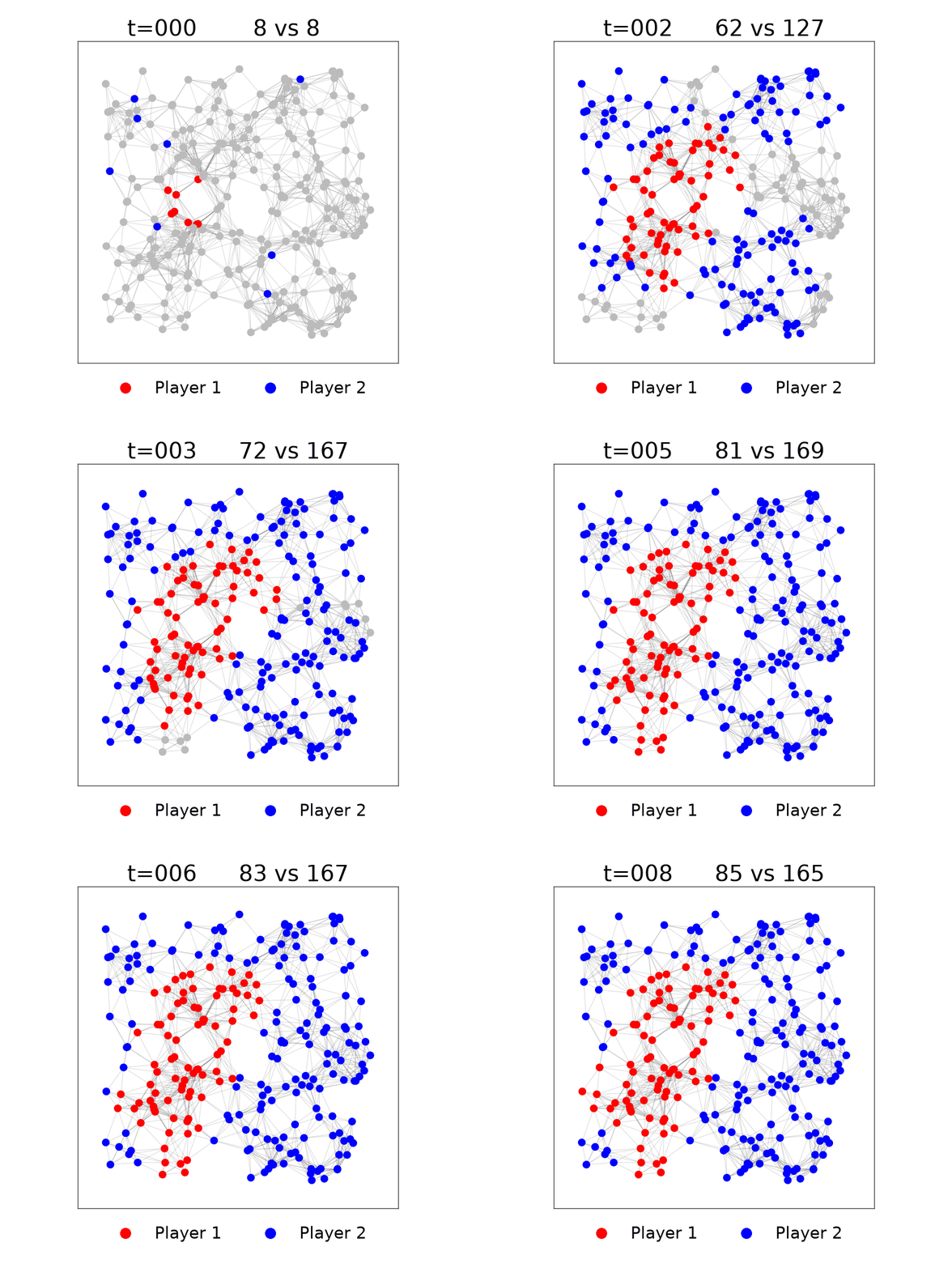 Here is an example game where Player 2 wins.
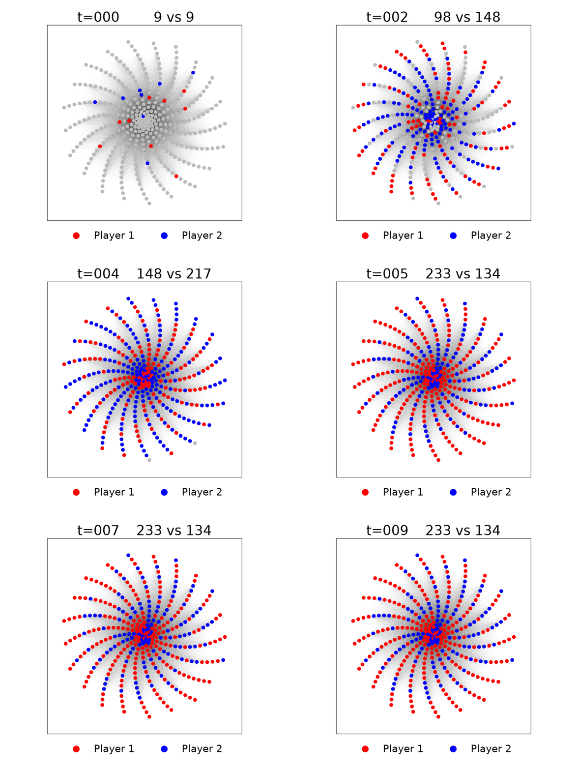 And here is an example that doesn't converge (in an ideal universe this would be considered a tie, but in the actual system it would end the simulation at a random timestep and therefore select either team as the winner with probability 1/2)
For the actual competition, all of the teams play against each other in a round-robin fashion. The graph is released (stored as an adjacency list), and then each team has 5 minutes to run whatever code is necessary and upload a set of seed nodes. After three days, with five rounds per day (each on a different type of graph), the team with the best total win-loss record is crowned the winner. For testing and research purposes, there were also a couple days of “pre-season” competition rounds where we could get used to the format and also collect samples of graphs/strategies that we might have to go against.
R&D
Take a second and think: how would you approach playing this game?
Even if you don’t really know much about graph theory, you might come up with the strategy of just choosing the nodes that have the most neighbors (i.e. the highest-degree nodes) to be your seeds. I’ll call this the “top-k” strategy. Intuitively, this makes sense, since you’re choosing the seed nodes that will infect the most nodes after one time step, and this will quickly cascade into infecting lots of nodes. This is a pretty decent strategy, but it’s far from the best. And in the later days of the competition, simulating top-k against all of the other teams showed that it would lose more often than not.
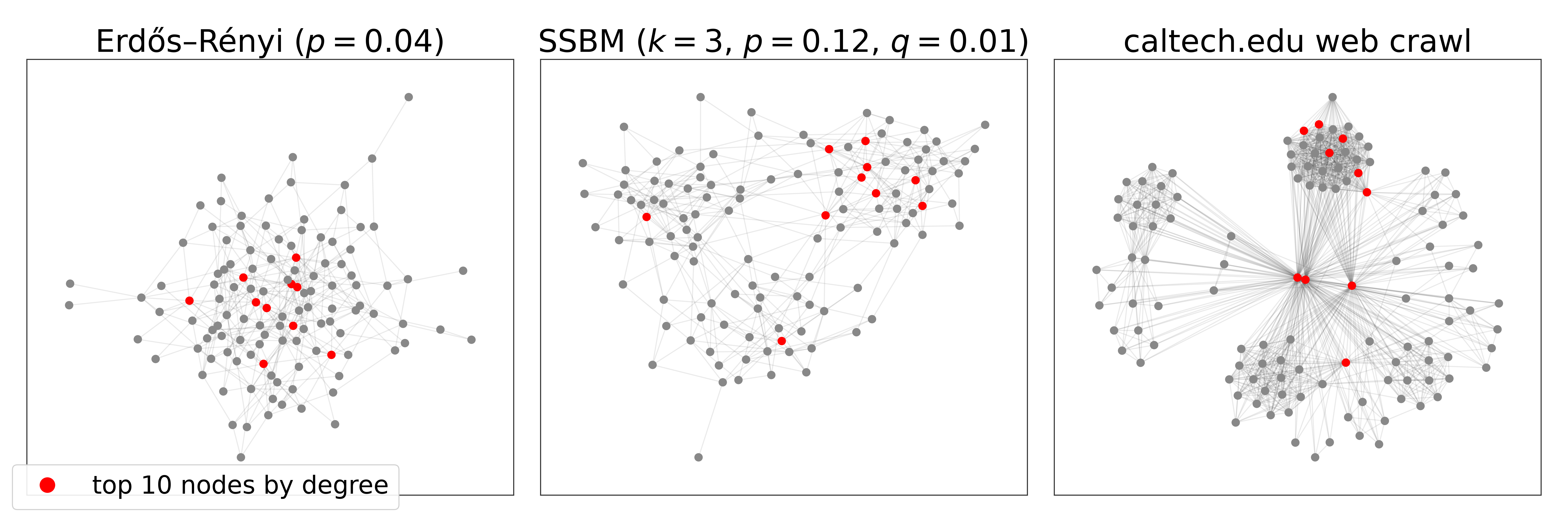 A few different example graphs and their highest-degree nodes
Ok, then can we come up with a smarter strategy using graph theory? Since some of the competition graphs are generated from models like Erdős-Rényi, Preferential Attachment, and Stochastic block model, we could also generate a selection of random graphs on which to test our strategies. I quickly wrote some Python scripts which could simulate different strategies against each other to produce a matrix of win/loss results. With some infrastructure in place, we were free to experiment to our heart’s content.
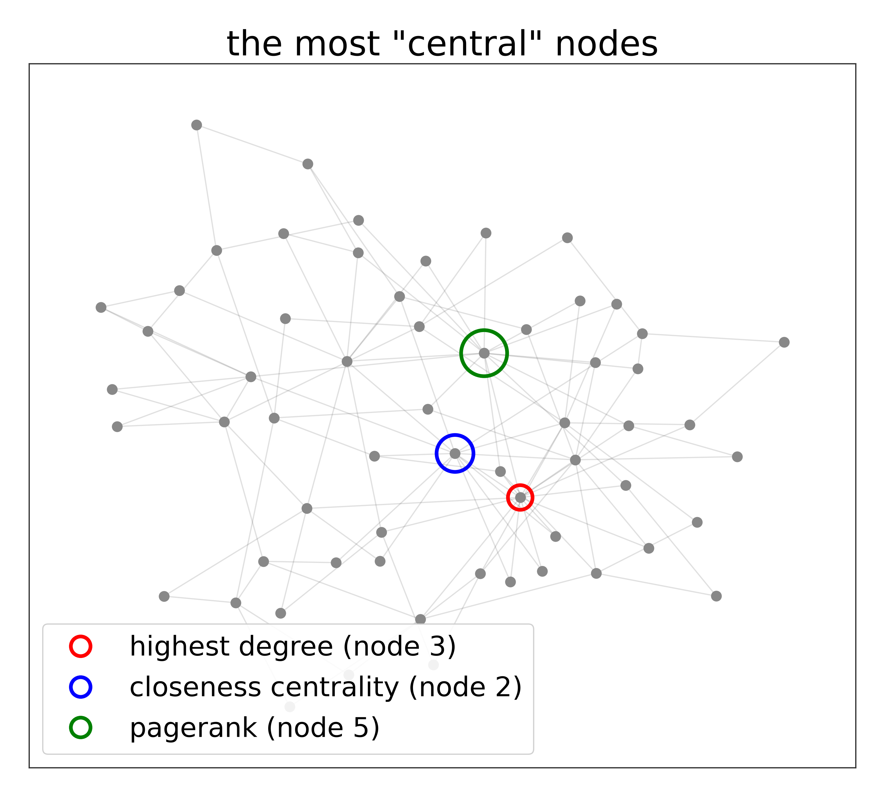
We looked at different measures of “centrality” in a graph. Intuitively, it would probably be good for a strategy to try and capture the “center” of a graph, right? Plus, if we spread out our seed nodes too much, then an opponent’s nodes could capture all of our nodes one-by-one. We tried using different measures of centrality like PageRank and Closeness centrality. Sometimes, this would win against top-k, sometimes not.
I also ended up plotting a bunch of node characteristics, like degree and level of centrality against each other. It turns out that degree and centrality are very correlated each other (at least on the random graphs we were provided with), so all of our methods that chose “central” nodes were basically just approximations of the top-k strategy. So we probably weren’t going to discover a magic “centrality measure” that would defeat other teams any better than top-k (though we tested every networkx centrality algorithm anyway just to make sure).
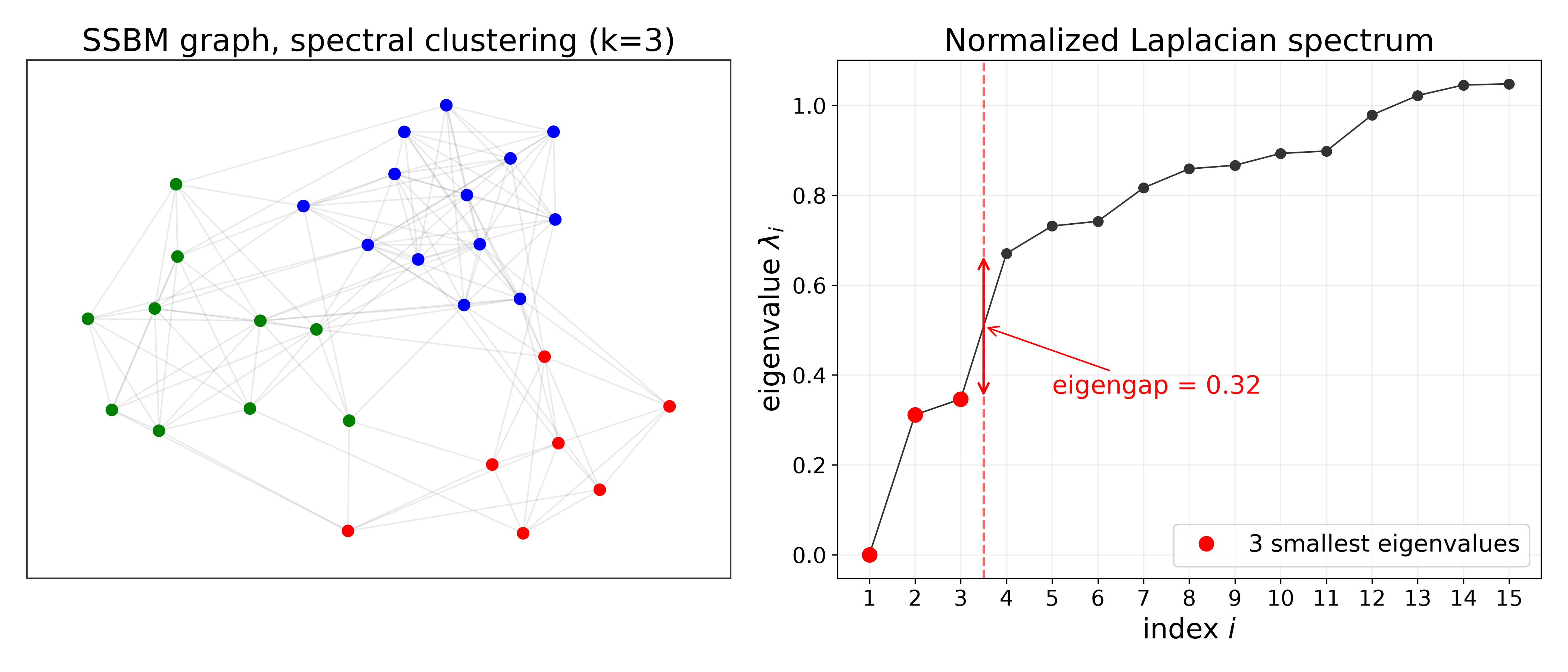
We can also analyze the graph using spectral clustering. Some of the graphs consisted of multiple clusters, so choosing the highest-degree nodes might split our seed nodes between two large clusters. But really, we only need to “capture” the largest cluster to win, since then we would end up with the most infected nodes.
We also tried mixed strategies. This was possible since each round really consisted of 50 simulations, and we were allowed to submit different seed nodes for each of these simulations (so randomized algorithms could be used). We tried taking the top 20 highest-degree nodes and then sampling 10 of them at random. Sometimes this beat top-k. Sometimes it didn’t.
One of my teammates looked into strategies designed to “counter” a different strategy and all sorts of crazy stuff inspired by papers in the field (the problem of “influence-maximization”).
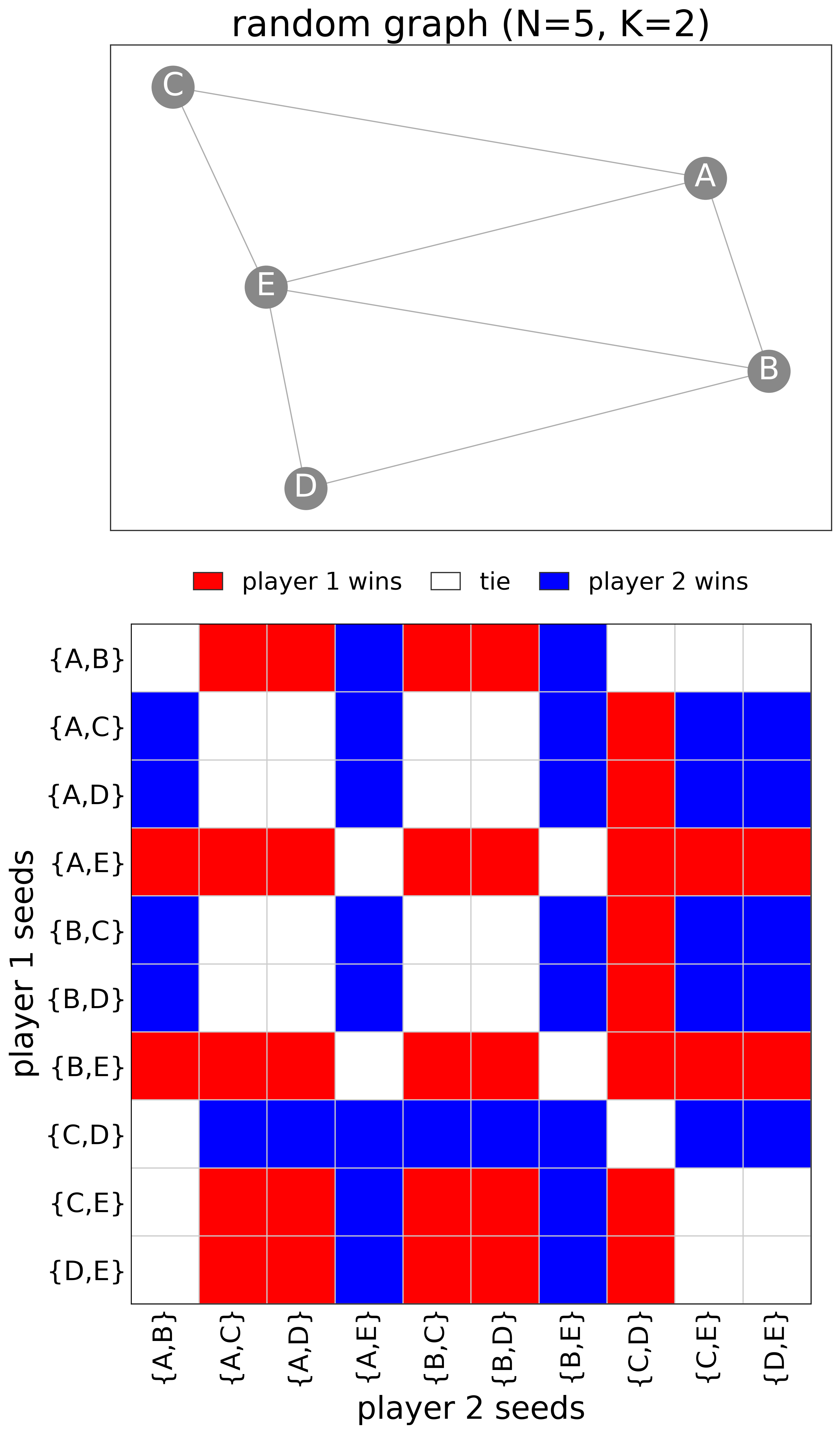 Brute-forcing a small graph, we see {A, E} and {B, E} are near-dominant seed nodes
Personally, I had also considered a brute-force method where you just test every possible set of seed nodes against every other set and choose the best. Asymptotically, I was looking at an algorithm with a time complexity of , or approximately , where is the size of the graph and is the number of seed nodes to choose. This also assumes that running each simulation takes a constant amount of time, which isn’t true (rather it seemed to scale up at least linearly with respect to the size of the graph). So anyway, that isn’t great.
Each graph had at least a couple hundred nodes, so naive brute force probably wouldn’t finish running before the heat death of the universe. Ok, let’s say we only look at the top, say, 30 highest-degree nodes, and choose 10 of those as seeds. That gives us games to simulate. For reference, even if we could simulate 1 billion games per second, it would still take 10 days to go through every match and pick the set of seed nodes that won the most times. And if any optimal set of seed nodes happens to choose a node that’s not in the top 30 highest-degree nodes, then we wouldn’t even find it.
After doing this computation, I figured there probably wasn’t a way to implement a brute-force strategy that would finish in a reasonable amount of time, especially not within the 5-minute time limit.
Brute-forcing it anyways
After a few days of pre-season and going crazy trying out many different types of strategies, we weren’t making much progress.
We were in the top 50% of the class but still far from the top of the leaderboard.
It felt like every new idea I tried either didn’t work against the other teams or lost to the simple top-k strategy.
While it wasn’t part of the grade, I really wanted to win the tournament.
But it wasn’t looking very good.
I decided to try and work more on the brute-force strategy. If we could brute-force a dominant strategy, or at least one that is close to dominant, then it would by definition win against almost every other team. And since each team is probably using heuristics like degree, centrality, clustering, etc, it’s unlikely anyone else could find a genuinely optimal strategy for every graph.
I went back to the runtime estimate from before and I thought: “well, 10 days is only a few orders of magnitude greater than 5 minutes.” Maybe with some optimizations, I could make it work.
Speeding up simulation
The first order of business was optimizing simulation as much as possible. By simulation, I mean implementing a function that takes a graph and two sets of seed nodes, then returns if the first or second set of seed nodes won. This is important because any brute-forcing code is going to be calling this function billions of times at least, so any bit of speed-up helps.
The Python example code provided from class implements simulation in a very naive way. It takes a graph in adjacency list form and iterates over each node, computing the “next” color by iterating over each of its neighbors and counting the number of red vs blue nodes. Then, it repeats this until the node colors stop changing, or a maximum number of iterations is hit. On my M1 MacBook Pro, it takes about 10 milliseconds to run a single 500-node simulation with 10 seed nodes.
However, I noticed that we could model the simulations in terms of matrix operations. Assuming each node in a given graph has been numbered from to , we can write the adjacency matrix as
And we can represent the state of each node as a column vector with entries:
This allows us to write out the “update” rule for the state vector as:
where represents the state at time . This works because multiplying the adjacency matrix with the state vector essentially “counts up” all the votes from a node’s neighbors, while the addition of 1.5 times the state vector adds in each node’s own vote and includes the tie-breaking behavior. Then, the sign function determines if there were more red votes or blue votes for every node, automatically setting them to be or as required. And since uncolored nodes have a state of , they don’t contribute to voting for either color. Then, we can repeat the update rule until the state vector stops changing and then check if the sum of the entries in this vector is positive or negative to figure out which team won.
This is a useful formulation since matrix operations are very fast on modern CPUs. Plus, the four components of the update rule: matmul, vector addition, multiplcation, and sign are all extremely parallelizable, so I would expect some very optimized SIMD implementations in whatever matrix backend numpy is calling into on my laptop.
Reimplementing the simulation code using numpy already yields a large speed-up — now, each simulation runs in about 0.2 milliseconds, which is 50x faster than before.
But I had another trick up my sleeve.

The Julia programming language was made for scientific programming, and it compiles from a Python-like language all the way down to native machine code to get really, really fast execution. Julia is genuinely one of my favorite programming languages (it’s also basically a lisp in disguise), and it’s an absolute cheat code if you want very fast code with very little effort.
Porting the code over didn’t give any speed-up by itself. However, a single line change makes it possible to swap out the standard dense matrices for sparse matrices, which come with their own crazy optimizations in the backend.
Additionally, since we found that most simulations terminated in less than 10 time steps, I just went ahead and hardcoded 10 time steps for every round, which 1) prevents run-away simulations that don’t converge from killing performance, 2) reduces the overhead from checking if the state vector had converged at each timestep, and 3) allows the compiler to unroll all of the matrix operations and inline more code, resulting in better performance. Then, with some Julia-specific optimizations, like preallocating structs and reusing them across iterations, I got rid of almost all heap allocations to minimize slow memory accesses.
In the end, I managed to get the time required to simulate a single round on a 500-node graph down to 25 microseconds on average. So that’s a 400x speed-up from the original Python implementation. And since this is just on a single-core, and each simulation can be run fully in parallel, I could theoretically get a throughput of up to 400,000 simulations per second just on my 10-core MacBook. Not bad, huh?
I also spent more than a few hours trying to see if I could take this even further and implement this search on a GPU for even more throughput, but I didn’t make much progress and eventually gave up.
Finding the best seeds
If the optimized simulation code was our V8 engine, then now we had to make the rest of the car.
Clearly, brute-forcing possibilities still won’t work, as we’re still nowhere near 1 billion simulations per second. What if instead we pit seed nodes against each other in a tournament, and take the winner repeatedly until we get the “best” set of seed nodes? This would be great for performance, as we’re reducing the problem to quickselect with , which is linear in the number of possibilities! But… it doesn’t work since the relation of “this set of nodes defeats this other set” is not a transitive property, at least in general. Claude comes up with this minimal counter-example:
You can verify that pitting each set of seed nodes against each other results in a cycle. It’s possible there’s some sort of semi-transitive property where if a set of nodes defeats, say, 50% of all other sets of seed nodes, then it’s likely to defeat a higher proportion of the remaining seed nodes than would be expected by chance. And maybe this could help with developing a tournament-based algorithm that can pick a good set of nodes in time or better. But we just went with the simpler (and asymptotically worse) approach of searching for the set of seed nodes which defeats the most other sets, i.e. maximizing dominance.
 the initial search idea
Now, for looking through sets of nodes. Even looking at the top 30 highest-degree nodes and choosing 10 of them is still too expensive ( rounds to simulate). At some point, we’re going to have to sacrifice optimality for speed. Looking at some of the pre-season rounds and the seed nodes which won most against the others, I noticed that the majority of winning seed nodes included the highest-degree nodes. So it wouldn’t be the worst idea to just, say, fix the 5 highest-degree nodes and then choose the other 5 from the remaining 25 highest-degree nodes. Because of the crazy combinatorial scaling, this results in only games to simulate, which could be done in just 2 hours with our theoretical throughput.
Then, we can also parallelize the problem in a smart way. On each thread, we can run a worker that, given a candidate set of seed nodes, loops through each possible opponent, counting up how many wins it achieves. Then, we can use a shared variable to keep track of how many wins the best candidate seed nodes have achieved so far, and if we test any set of nodes which loses too many times, we can immediately stop the worker and move on to a different candidate. This helps a lot, since it seems in practice we could very quickly find a set of seed nodes that wins against, say, 95% of all the other possible sets of seed nodes, and so we can cull any candidate as soon as it loses to just 5% of the total number of possible sets of seed nodes. So this massively decreases the number of games we have to simulate.
On my laptop, the runtime was now down to 5-10 minutes, depending on the graph. And when I ran the brute-forcing script on my friend Sam’s server with an Intel i9-14900K (24 core, 32 thread), the runtime was halved to about 3-6 minutes, so we could now feasibly use this strategy in the competition.
Fine-tuning
By the time we got the brute-force strategy working, it was actually already the second day of the three-day competition. We were in 5th place (out of around 12) after the first day, using our old strategies. And as soon as we used the brute-force seed nodes, our ranking jumped up to being tied for first. This was a massive improvement, but I wasn’t going to let chance dictate if we won first place or not.
While we did well on most of the graphs, there was one in particular where we lost to all but two of the opposing teams. When I downloaded and visualized the seed nodes we lost to, the main thing I noticed was that many of the other teams chose nodes with a lower degree than expected, and some of the top 5 highest-degree nodes weren’t even chosen, while we forced our seed nodes to include those. So this is our assumption from above coming back to bite us.
If we extended our initial “search” to include any more low-degree nodes, we would be looking at a 50% increase in computation required per additional node. And if we fixed the top 6 highest-degree nodes instead of 5, we could increase our search to 34 lower-degree nodes instead of 25 before hitting the same computational wall. But this also doesn’t fix the problem of finding solutions that don’t even include the few highest-degree nodes at all. We were stuck.
 the secondary search
But that’s when one of my teammates came up with a genius idea: what if we ran a second search in which we look through lots of low-degree nodes and try to swap them into our initial solution? This way, we vastly expand the search space and can find solutions in which it’s better to take a low-degree node which happens to be positioned better than a high-degree node, effectiovely un-fixing the top 5 highest-degree nodes. This is also not very computationally intensive, since if we limit the search to swapping out just 2 of the original seed nodes with any of the next 55 highest-degree nodes, then it only requires computing at most simulations, which is on the same order of magnitude as the initial brute-force search. And thanks to the same optimizations mentioned before, this would only add at most a few minutes into the total runtime of the program.
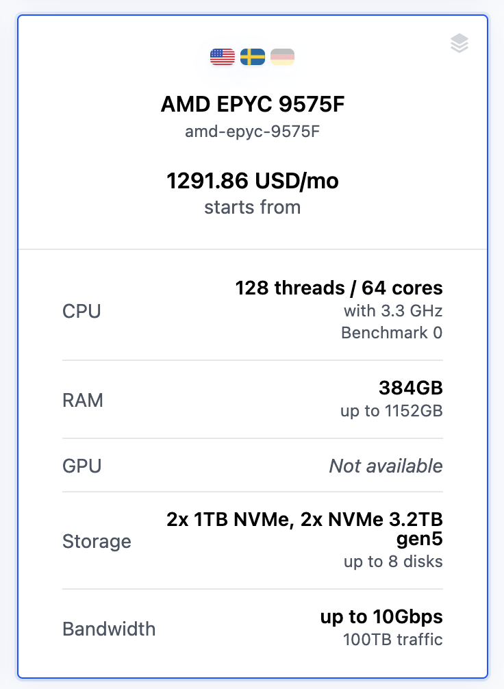
Just to absolutely make sure we could run all of our brute-forcing within the 5-minute time limit, I rented a server from Cherry Servers (not sponsored, I just like their services) with an AMD EPYC 9575F (64 core, 128 thread) for about $3 per hour. This decreased our brute-forcing runtime all the way down to 1-2 minutes per graph, way under the time limit.
I also experimented with a slightly different strategy, where instead of using degree to do the initial ranking of nodes, I could use a different heuristic. I computed a metric which I coined “solo winnability”, in which I pitted every single node against every other and then ranked them by the number of wins. This could be run very quickly, and my logic was that in tough matchups where both teams pick very similar nodes, most of them will collide and disappear, possibly leaving just one or two distinct nodes per side that go on to win or lose. So maximizing “solo winnability” would be looking at nodes which would perform well if they were the “last node remaining”. This helped us win some games that we would not have otherwise, but it didn’t do quite as well as the normal brute-force strategy in past rounds (simulated on historical game data).
But since our strategy already ran in 1-2 minutes, we had enough time to run both the original version of the brute-forcing strategy and this modified solo-winnable strategy to generate two sets of seed nodes, and then we could pit these two against each other and take the winner. And worst case, if the second strategy doesn’t finish running in time, we could always just comfortably use the first solution.
And with all of this, we were ready for the final day of the competition. Keep in mind that I basically ignored all of my other classes and just focused all of my efforts on developing this strategy, fine-tuning parameters, and making sure everything worked properly until like 4am multiple days in a row.
 yippee
Long story short… we won!
Conclusion
So, it turns out that the actual graded part of this project was winning against two of the TA bots in the pre-season competition. And we actually didn’t achieve that… since most of the development I described was in the days leading up to and during the official three-day competition. This meant our overall project grade was capped at 90 percent 😭😭😭
But on the final project report, we asked if winning the competition could make up for not beating the TA bots earlier, and luckily, the graders were nice enough to give us the points! Funnily enough, the professor seems to have predicted my behavior when he came up with the assignment…
Are class competitions damaging?… because many of the students get engrossed in the competition, they end up spending a considerable (maybe ridiculous) amount of time on them! This is despite the fact that grades are not affected by the competition… But, at the same time, many of those teams were the ones that enjoyed it the most — and it certainly was a memorable learning experience for them.
~Adam Wierman (2014)
In another blog post, Wierman explains that there isn’t much literature on this exact problem of competing epidemics, and he figured that by throwing enough undergrads at the problem, we might be able to approximate an equilibrium strategy. I think he’s moved on from the research topic at this point, but I think it’s funny that was the original motivation for the class project.
All throughout conducting this project, in the back of my mind, I was thinking about Rich Sutton’s essay The Bitter Lesson. The very first sentence in the essay: “The biggest lesson that can be read from 70 years of AI research is that general methods that leverage computation are ultimately the most effective, and by a large margin.” In summary, the essay points out that over and over again historically, smart brute-force search algorithms almost always perform better than hand-tuned techniques based on “human knowledge” as computation becomes cheaper and more widespread. People seem to love arguing about this essay on Hacker News, so I won’t expand too much on it here, but I’ll say that I can’t help but notice that it seems to have manifested itself yet again in this competition.
I think this blog post is long enough at this point, so I’ll go ahead and end it. Hopefully you enjoyed reading! Shoutouts to my awesome teammates Miles and Alexa.
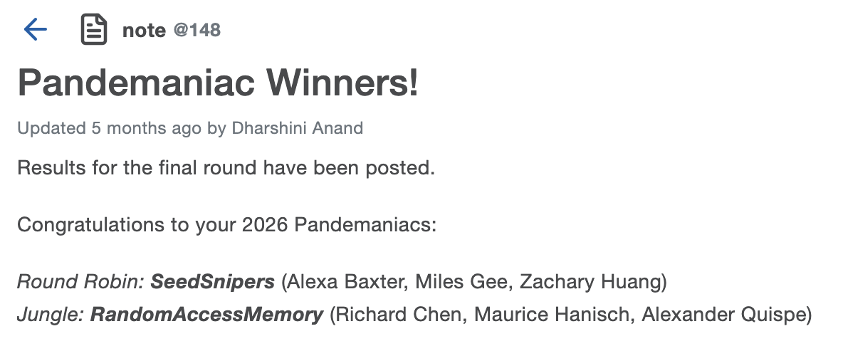
P.S. There was also a whole other gamemode in which every team faced off on the same graph, called Jungle, as opposed to the round-robin 1v1 games. We didn’t focus very much on this mode (I think there was vastly, vastly more variance in the results lol).


Zachary W. Huang © 2021-2026